Helmholtz equation
Contents
Helmholtz equation#
This tutorial demonstrates how to solve the Helmholtz equation (the eigenvalue problem for the Laplace operator) on a box mesh with an opposite inlet and outlet. Specifically, it shows how to:
obtain the variational formulation of an eigenvalue problem
apply Dirichlet boundary conditions (tricky!)
use
SLEPcandscipyto solve the generalized eigenvalue problem
Additionally, different SLEPc solvers are compared and a benchmark is performed against AVSP (our in-house tool to solve this kind of problems).
Formulating the problem#
Our goal is to find \(u \neq 0, \lambda \in \mathbb{R}\) such that
Following the usual approach (remember FEniCS needs the variational formulation of a problem), we multiply both sides by a test function \(v\) and integrate by parts. Our problem is to find \(0 \neq u \in V, \lambda \in \mathbb{R}\) such that
Notice our eigenvalue problem is now a generalized eigenvalue problem of the form:
This is very different from the problems most commonly solved in FEniCS, as \(u\) appears in both sides of the equation, and therefore the problem cannot be represented in the canonical notation for variational problems: find \(u \in V\) such that
You can find more details about the formulation in these delightful notes from Patrick Farrell.
A simple solution#
Creating the mesh#
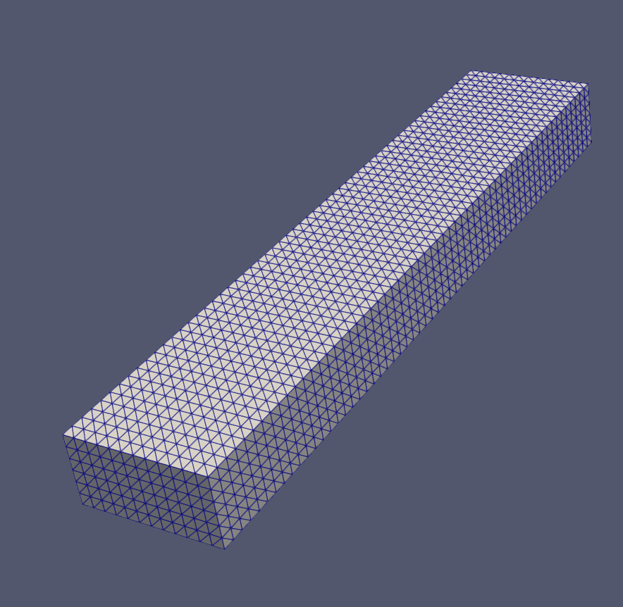
For this example we will create a simple box mesh.
from dolfin.cpp.generation import BoxMesh
from dolfin.cpp.generation import Point

N = 60
lx, ly, lz = 0.2, 0.1, 1.0
mesh = BoxMesh(Point(0, 0, 0), Point(lx, ly, lz), int(lx*N), int(ly*N), int(lz*N))
This is how it looks:
Translate the problem formulation into code#
The equations shown above are reflected in the code as follows:
from dolfin.function.functionspace import FunctionSpace
from dolfin.function.argument import TrialFunction
from dolfin.function.argument import TestFunction

from ufl import inner
from ufl import grad
from ufl import dx

V = FunctionSpace(mesh, 'Lagrange', 1)

u_h = TrialFunction(V)
v_h = TestFunction(V)

a = inner(grad(u_h), grad(v_h)) * dx
b = inner(u_h, v_h) * dx
Assemble the matrices and apply boundary conditions#
The assembling of the matrices and application of the boundary conditions is the most sensitive part of this tutorial. The main reason is that it is not advised to remove rows and columns of matrices, as it is an inefficient operation (remember we are dealing with sparse matrices). To circumvent that, several alternatives to impose Dirichlet boundary conditions exist. Independently of the chosen strategy, the key point is to preserve symmetry in both matrices, as the available eigensolvers are better suited for symmetric problems (and it is a pitty to loose such a nice property!).
Our strategy consists in zeroing-out the rows and columns corresponding to “Dirichlet degrees of freedom” and assign \(\alpha\) and 1 to the corresponding diagonals, for \(A\) and \(M\), respectively. \(\alpha\) is the value that meaningless (artificial) eigenvalues will take. If you want to avoid them, just choose a value that is outside the desired spectrum.
Let’s now perform the assembly:
from dolfin.cpp.la import PETScMatrix
from dolfin.fem.assembling import assemble

A = PETScMatrix(V.mesh().mpi_comm())
assemble(a, tensor=A)

B = PETScMatrix(V.mesh().mpi_comm())
assemble(b, tensor=B)
Notice we are using PETSc matrices, which are sparse. These data type is required to work with SLEPc later.
For the application of boundary conditions, we start by collecting the Dirichlet dofs:
bc_dofs = []
for bc in bcs:
    bc_dofs.extend(list(bc.get_boundary_values().keys()))
Here, bcs is a list with Dirichlet boundary conditions. We are fixing the two faces perpendicular to \(z\) axis.
Finally, we use directly a method available in the PETSc matrix object to apply our chosen strategy (FEniCS equivalent method does not work in parallel):
A.mat().zeroRowsColumnsLocal(bc_dofs, diag=diag_value)
B.mat().zeroRowsColumnsLocal(bc_dofs, diag=1.)
Note that homogeneous Neumann boundary conditions are very simple to treat: do nothing!
What to do with these matrices?#
FEniCS considers SLEPc the go-to library to solve eigenvalue problems. Nevertheless, after assembling the matrices, we can choose any solver we want (including our own!). A good starting point is the most commonly used scientific libraries numpy and scipy. numpy provides machinery to solve “normal” eigenvalue problems, but it is not able to solve generalized eigenvalue problems. Besides, the lack of sparse data structures clearly shows its inability to scale (you cannot go that far with dense matrices). On the other hand, scipy provide solutions both for dense and sparse matrices.
Let’s solve it with scipy then:
import scipy

A_array = scipy.sparse.csr_matrix(A.mat().getValuesCSR()[::-1])
B_array = scipy.sparse.csr_matrix(B.mat().getValuesCSR()[::-1])

k = 20  # number of eigenvalues
which = 'SM'  # smallest magnityde
w, v = scipy.linalg.eigh(A_array, B_array, k=k, which=which)
scipy.sparse.linalg.eigsh relies on ARPACK’s implementation of the Implicitly Restarted Lanczos method.
On the other hand, the basic usage of SLEPc is also very simple:
import numpy as np
from dolfin.cpp.la import SLEPcEigenSolver

# instantiate solver
solver = SLEPcEigenSolver(A, B)

# update parameters
solver.parameters['solver'] = 'krylov-schur'
solver.parameters['spectrum'] = 'smallest magnitude'
solver.parameters['problem_type'] = 'gen_hermitian'
solver.parameters['tolerance'] = 1e-4

# solve
n_eig = 20
solver.solve(n_eig)

# collect eigenpairs
w, v = [], []
for i in range(solver.get_number_converged()):
    r, _, rv, _ = solver.get_eigenpair(i)
    w.append(r)
    v.append(rv)

w = np.array(w)
v = np.array(v).T
Our preliminary studies show scipy is not competitive with SLEPc for large problems.
This paper presents open-source libraries capable of solving eigenvalue problems (focus is generalized non-hermitian eigenvalue problems), which may also be explored: LAPACK, ARPACK, Anasazi, SLEPc, FEAST, z-PARES. Their summary of each library (and algorithms) is worth reading.
What SLEPc offers?#
Above, we’ve used SLEPc without much thinking. Yet, it offers several algorithms to solve eigenvalue problems, including: power iterations, subspace iterations, Arnoldi, Lanczos, Krylov-Schur (default), Jacobi-Davidson and Generalized Davidson.
FEniCS documentation is outdated (it is a good idea to peek into the code to know what is really available). These are the possible arguments for solver.parameters['solver']: power, subspace, arnoldi, lanczos, krylov-schur, lapack, arpack, jacobi-davidson, generalized-davidson. You can find here further information about each option.
We are simply relying on the methods FEniCS exposes from SLEPc library. If we want to go further, we can also use slepc4py, which are the bindings for SLEPc and provide much more flexibility.
The following picture shows how each algorithm compare in terms of performance for the problem described above (changing the mesh size):
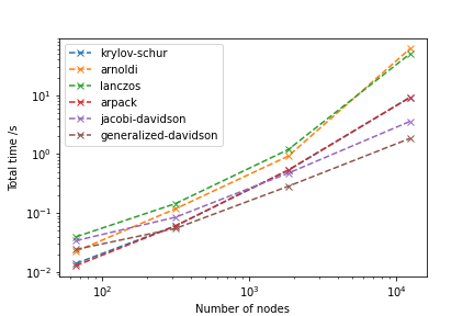
As you can see, generalized-davidson outperforms all the other (the options not tested are not suitable for this problem). In fact, it allows to solve a problem with approximately 100k degrees of freedom in about 13 seconds (very dependent on parameters such as tolerance). From this number of degrees of freedom on, the weakest point of the chosen strategy is not anymore the solver, but the assembling step (solution: go parallel).
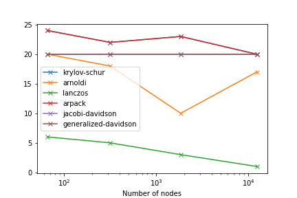
It is also important to check the number of converged solutions (we ask for 20):
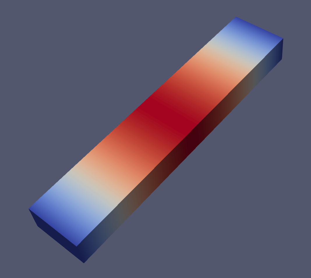
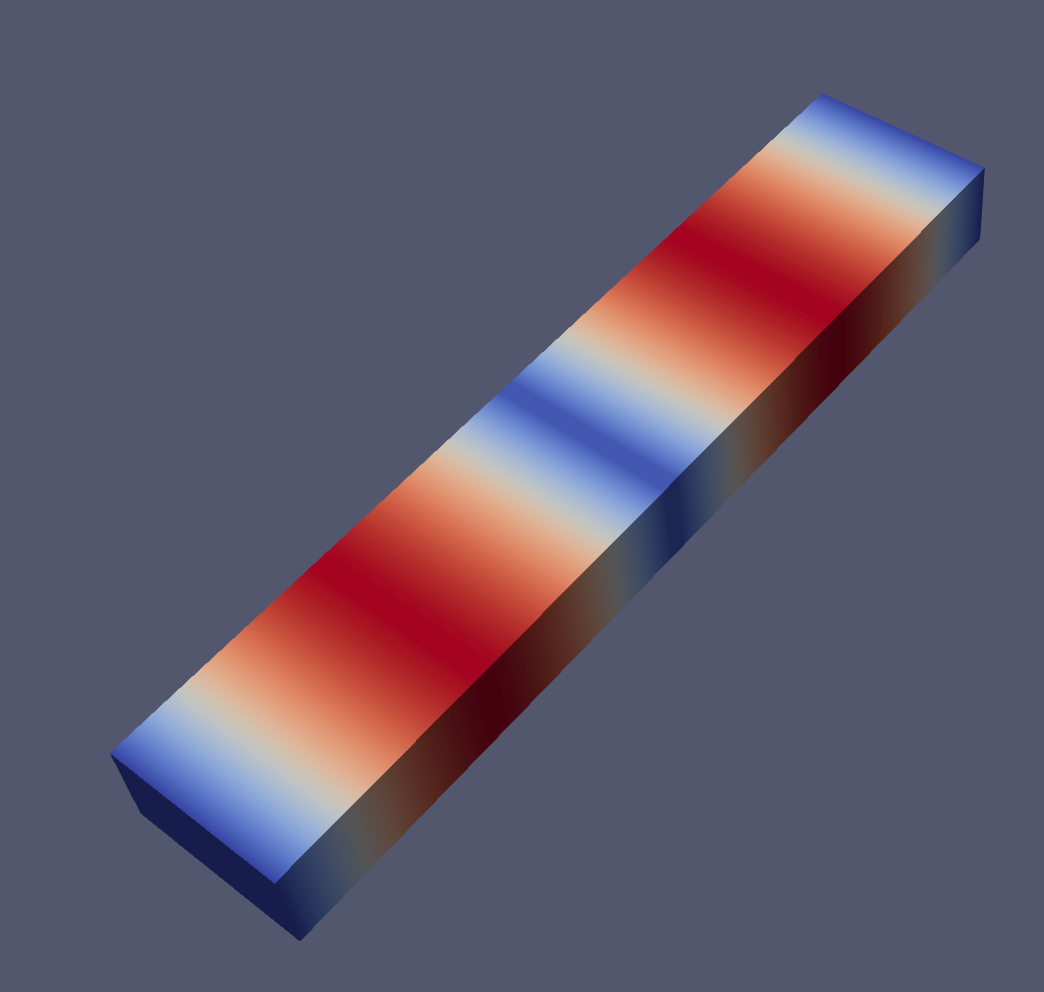
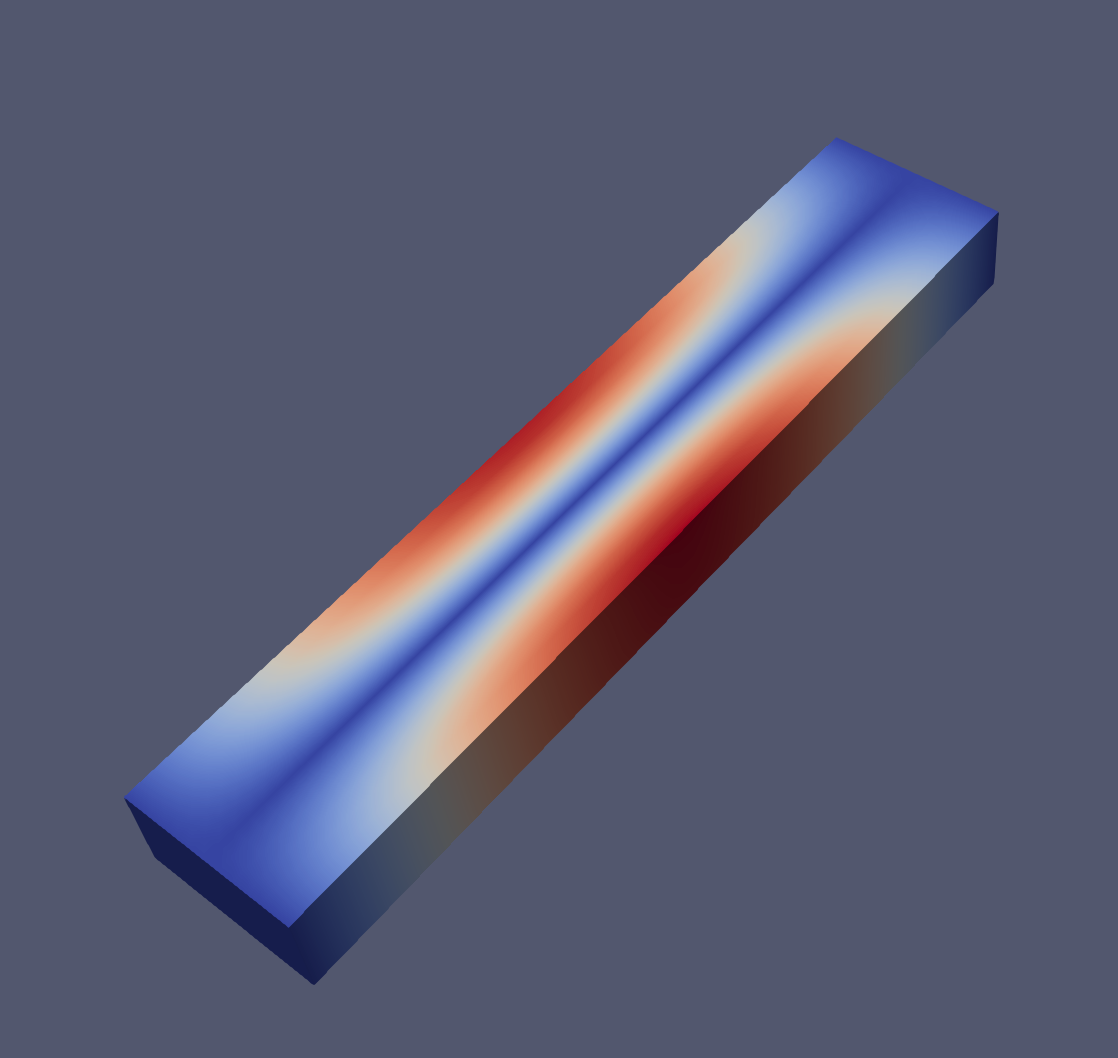
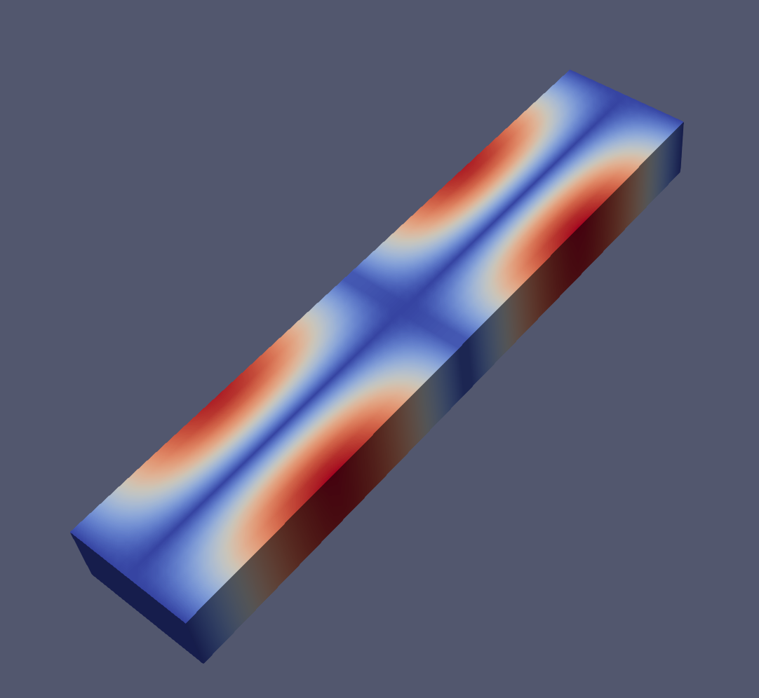
Modes#
And an example of the modes 1, 2, 6 and 7 visualized with paraview:
Closing remarks#
Have you seen how simple it is to solve an eigenproblem with FEniCS? An example script can be found here.