How to define and apply boundary conditions?
Contents
How to define and apply boundary conditions?#
Note
This tutorial covers the application of different kind of boundary conditions (Dirichlet, Neumann and Robin) following different strategies (from the basic use of functions to define boundaries, to more complex approaches as using compiled subdomains). Please refer to it for a more detailed overview.
By definition, Dirichlet boundary conditions represent degrees of freedom (dofs) for which we already know the solution. Therefore, we essentially need to provide FEniCS with the corresponding dofs or a way to find the corresponding dofs (e.g. a function that defines if a point belongs to the Dirichlet boundary), and the corresponding values.
Homogeneous Neumann boundary conditions are naturally handled by the finite element method (meaning boundaries without explicitly defined boundary conditions are considered homogeneous Neumann). Inhomogeneous Neumann boundary conditions are represented by an additional term in the variational approach (which will be converted in an additional vector belonging to the righ-hand side of the variational problem, i.e. to the linear form).
Note
In the strategy explained above, Dirichlet boundary conditions are strongly imposed. An alternative is to impose them weakly.
Dirichlet boundary conditions#
Define (a simple example)#
Imagine we want to apply a Dirichlet boundary condition to the left edge of a unit square.
First, we need to define a function that identifies if a given point belongs to the edge:
from dolfin.cpp.math import near

def boundary(x, on_boundary):
    return on_boundary and near(x[0], 0.)
x is an array with the coordinates of the point. on_boundary is a boolean that is True if the point belongs to the boundary. near compares two floats (by default a tol= 3e-16).
Then, we create a Dirichlet boundary condition object:
from dolfin.fem.dirichletbc import DirichletBC

bc = DirichletBC(V, u_D, boundary)
V is the function space and u_D the desired value.
More complex boundaries are hard to define using simple mathematical expressions. Boundary markers are then the simplest way to identify them (check this out for more information).
Apply: black-box case#
The black-box approach to apply Dirichlet boundary conditions consists in simply passing them to the solve function:
solve(a == L, u, bc, solver_parameters=solver_parameters)
If you are solving a symmetric problem, ensure to pass symmetric = True in solver_parameters, in order to keep symmetry after the application of boundary conditions and use a convenient solver (more information on how it impacts solver choice here).
Apply: breaking symmetry#
On the other hand, it is usually useful to apply boundary conditions directly on assembled matrices. The simplest (yet not recommended) way to do it consists in zeroing-out rows that represent Dirichlet dofs. That’s the task performed by bc.apply.
As example, let’s take the bilinear form of Poisson equation:
which is translated in ufl language as (V is the function space):
from dolfin.function.argument import TrialFunction
from dolfin.function.argument import TestFunction

from ufl import dot
from ufl import grad
from ufl import dx

u_h = TrialFunction(V)
v_h = TestFunction(V)

a = dot(grad(u_h), grad(v_h))*dx
To assemble the matrix:
from dolfin.fem.assembling import assemble

A = assemble(a)
Finally, to apply boundary conditions:
for bc in bcs:
    bc.apply(A)
A pictorial representation of the assembled matrices before (left) and after (right) boundary condition application is shown next (yellow represents non-zero elements).
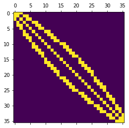
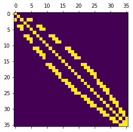
The drawback of this approach is that initially symmetric matrices become non-symmetric (e.g. take a look to first row and column)… and symmetry is a property we want to keep at all costs!
In the right-hand side, this solution consists in replacing the components corresponding to Dirichlet dofs by the desired values (the Dirichelet dofs equations become \(u_i = u_{D_i}\)).
Apply: keeping symmetry#
A better way to apply boundary conditions is to use assemble_system, since it keeps symmetry when applying boundary conditions. For that, we need both the bilinear and linear forms of the problem. For Poisson equation, the linear form is:
which is translated in ufl language as (V is the function space):
from dolfin.function.constant import Constant
from ufl import dx

f = Constant(-6.) # just as example
L = f*v_h*dx
To assemble the matrix and the vector:
from dolfin.fem.assembling import assemble_system

A, b = assemble_system(a, L, bcs)
This way, A is kept symmetric, as the next pictorial representation shows.

assemble_system incorporates (in a symmetric way) the boundary conditions directly in the element matrices and vectors, prior to assembly (check out Logg’s book to learn more about the assembly algorithm). The advantage of taking care of boundary conditions at element level is that the process of eliminating whole rows and columns is more efficient (than when matrices are stored in compressed row format).
Apply: keeping symmetry but varying right-hand side (advanced)#
For time-dependent problems, it is usually convenient to assemble the left-hand side only once (as the assembly operation can be costly for large problems). Following the “breaking symmetry” approach, it is trivial to achieve this goal, as the application of boundary conditions is done independently for each equation side. For the “keeping symmetric” approach, things get slightly more complicated: it is necessary to keep track of an additional vector that stores the results of the elimination process.
The process of assembling the left-hand side is:
dummy = Constant(0.)*v_h*dx  # integrates to zero

A, dummy_vec = assemble_system(a, dummy)
Mathematically, this dummy vector is \(\sum_i u_{D_i} a_i\), where \(u_{D_i}\) represents the value of the Dirichlet boundary condition at dof \(i\) and \(a_i\) represents the \(i\) column of matrix \(A\) after zeroing-out all the Dirichlet dofs rows.
To obtain the right-hand side:
b_tmp = assemble(L)

b = b_tmp + dummy_vec
for bc in bcs:
    bc.apply(b)
bc.apply(b) is performed to ensure the correct values at Dirichlet dofs components.
Note
Althought quite general, this example ignores time-dependent Dirichlet boundary conditions. Can you see what needs to change? (Tip: writing \(u_D\) as \(u_D(x, t) = u_D(t) u_D(x) + u_D(t) + u_D(x)\) can help)