Heat equation in the trapped vortex case
Contents
Heat equation in the trapped vortex case#
In this tutorial, the goal is to show how you can take an existing CERFACS mesh (created with e.g. hip) and solve the time-dependent heat equation problem. It shows how to:
convert the mesh in a DOLFIN’s-friendly format
apply boundary and initial conditions
translate the variational formulation into code
solve the problem relying on different solvers
parallelize your code
The heat equation tutorial found in Langtangen’s 2017 book (web version) is closely followed. You should go there if you struggle with any of the steps.
Formulating the problem#
This is the partial dfferential equation we are trying to solve:
Since it is a time-dependent problem, we need to make a choice about the time-integration scheme. Choosing a backwards Euler scheme:
we can transform the initial problem in a sequence of linear variational problems: find \(u^{n+1} \in V\) such that
for all \(v \in V\).
(The usual steps of multiplying by a test function \(v\), integrating both sides in the whole domain, and integrating by parts to reduce the maximum derivative in the formulation are performed.)
Note
We can rewrite the above variational problem as:
which can be very easily translated into matrix notation:
This last formulation may show better how easy it is to implement any other time-integration scheme, as the general form for this problem is given by:
After we have the variational problem formulated, implementing it in FEniCS is straightforward.
A first working simulation#
Convert and load the mesh#
In this example, we start with a typical hip xmf file. Then, we convert it to dolfin’s required format following the procedures shown in How to convert a CERFACS mesh?.
Recall that at the end of this process we have a mesh object (named mesh in this tutorial code snippets), the boundary markers (boundary_markers), and a list with patch labels (patch_labels).
Within a notebook, the mesh can be visualized by simply running a cell with the mesh object.
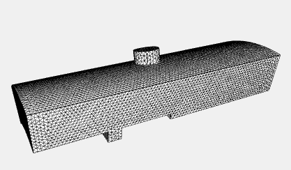
This mesh has 34684 nodes.
Define the function space#
As seen in the problem formulation, a variational problem consists in finding the solution that lies in the trial space. To define a function space (which will be then used to build test and trial functions), the element family and degree need to be specified (look here for the available options). For a simple Lagrange space of degree 1:
from dolfin.function.functionspace import FunctionSpace

V = FunctionSpace(mesh, 'Lagrange', 1)
Define the boundary conditions#
In this case, we specify Dirichlet boundary conditions at the inlet and the outlet (\(u=300\)). All the other boundaries assume null flux. Knowing that:
>> patch_labels
['Inlet',
 'Outlet',
 'PerioLeft',
 # ...
]
the boundary conditions can be applied as follow (check out How to define Dirichlet boundary conditions using patches?):
from dolfin.function.constant import Constant
from dolfin.fem.dirichletbc import DirichletBC

u_inlet, u_outlet = Constant(300.), Constant(300.)

bcs = [DirichletBC(V, u_inlet, boundary_markers, 0),
       DirichletBC(V, u_outlet, boundary_markers, 1)]
Here some aspects worth noticing:
Constantspecifies a constant value for all the nodes at the corresponding boundary. We could have used afloatinstead. Nevertheless, this way gives you already a hint on how to set up non-constant boundary conditions: useExpressioninstead.All the boundary conditions are stored in an array that will then be passed to the solver.
Define the initial condition#
Since this is a time-dependent problem, we have to specify an initial condition.
from dolfin.function.expression import Expression
from dolfin.function.function import Function

c = 0.2 / 2.  # (x_max - x_min) / 2.
param = u_inlet.values()[0] / c**2  # 300. / c**2

u_initial = Expression('param * (x[0] - c) * (x[0] - c)',
                       degree=2, param=param, c=c, name='T')

u_n = Function(V, name='T')
u_n.interpolate(u_initial)
A small caveat: string expressions must have valid C++ syntax.
u_n represents our initial condition (a parabolic temperature field). We are getting it via interpolation. Alternatively, this could have been solved by projection (by turning the initial value problem into a variational problem), via projection method.
Translate the problem formulation into code#
The last setup step is to “translate” the variational mathematical formulation into code. The unified form language (UFL) library is of great help here.
from dolfin.function.argument import TestFunction
from dolfin.function.argument import TrialFunction
from dolfin.function.function import Function
from dolfin.function.constant import Constant

from ufl import grad
from ufl import dx
from ufl import dot

u_h = TrialFunction(V)
v_h = TestFunction(V)
f = Constant(0.)

a = u_h*v_h*dx + dt*dot(grad(u_h), grad(v_h))*dx
L = (u_n + dt*f)*v_h*dx
Don’t forget to define dt first.
T = 0.05  # final time
num_steps = 20  # number of time steps
dt = T / num_steps
Solve the problem#
And finally we arrived to the last destination. Nevertheless, let’s not go there so fast… let’s start simple. If our problem did not depend on time, this is how we would solve it:
from dolfin.function.function import Function
from dolfin.fem.solving import solve

solver_parameters = {
    'linear_solver': 'lu',  # chosen by default
    'preconditioner': None,
    'symmetric': True,
}

u = Function(V, name='T')
solve(a == L, u, bcs, solver_parameters=solver_parameters)
Simple, isn’t it? The results can also be store in a format amenable to paraview or other visualization tools (we strongly recommend PyVista):
import os
from dolfin.cpp.io import XDMFFile

file = XDMFFile(os.path.join('outputs', 'trappedvtx_heat_eq.xdmf'))
file.write(u)
Nevertheless, our problem does depend on time. This means we will have to perform a loop and update the time-dependent variables each cycle:
file.parameters['flush_output'] = False
file.parameters['functions_share_mesh'] = True
file.parameters['rewrite_function_mesh'] = False

# store initial solution
t = 0.
file.write(u_n, t)

u = Function(V, name='T')
for n in range(num_steps):

    # update current time
    t += dt

    # compute solution
    solve(a == L, u, bcs, solver_parameters=solver_parameters)

    # save to file
    file.write(u, t)

    # update previous solutions
    u_n.assign(u)
Regarding file parameters: flush_output enables to open the result file before the loop is finished; with function_share_mesh only one mesh is used for all function at a given time step (imagine the case two or more variables are computed); rewrite_mesh_function is similar to function_share_mesh, but for different time steps (i.e. if False, mesh is only saved once). (Information found here.)
And this is all. You can now go to paraview and play with your results.
What about a fastest solver?#
But wait… have you followed all the steps and now you are very unhappy with the performance of the solver? Are you wondering why such a slow code would be worth to look at? Well, the slowness is your fault… you are solving a medium-size problem with LU decomposition, which is the default solver in FEniCS and which is suggested for problems with “a few thousand of unknowns”. Just do the following, and your doubts will start vanishing.
solver_parameters = {'linear_solver': 'cg',
                     'preconditioner': 'ilu',
                     'symmetric': True}
We have just changed the solver to a Krylov subspace method and our performance increased about ten-fold. In the implementation, only the line containing the solver changes, since now we want to have control over its parameters.
Let’s go parallel#
DOLFIN supports parallel computing through MPI and is supposed to perform well in massively parallel supercomputers. It is designed such that the parallel simulations use the same code as for serial computations. The difference is the way you run your script:
mpirun -n <n_cpus> python <your_script>
Don’t forget to use a linear algebra backend that supports parallel operations (e.g. PETSc).
Multithreading was previously supported, but it was removed around 2014.
Closing remarks#
There are several ways to implement a problem in FEniCS. The example presented here follows a script-based way, which is easier to read in a blog post. Nevertheless, if you start using FEniCS often, you will crave for creating your own objects that encapsulate the tasks you perform recurrently (and which are not particular to your very specific problem). If you ever felt such a crave, you are in the right path.
As this process seemed long to you? Just look how short the script is with all the pieces we have used above.
What to do next?#
Assembling matrices can be expensive. Can you see a better way to perform the time-dependent loop?
What about different time-schemes? Can you take the general matrix formulation and simply implement a forward Euler scheme? And a higher-order scheme? How does the time-scheme influence the performance and the accuracy of the results?